MOORING BERTHING LOAD CALCULATION ON JETTY OR WHARFSIDE

WHARF MOORING SYSTEM DE PHILOSOPHY

This article is to provide the Mooring and berthing load calculation on Bollards and Fenders. Assuming Bollards and Fenders are installed at Piles, Forces can be transferred to Piles for Pile design load calculation Wharf or Jetty Mooring arrangement.

Wharf shall moor the barges and tug boats of various sizes on both sides of wharfs. This Wharf structure are designed with steel mono-pile, with steel pile head platforms installed. The wharf will be fitted with Cone Type or typical tyre fenders on the Pile to protect against impact and facilitate landing of ships.

Mooring system to wharf side shall comprise of Braided Nylon Ropes and mooring bits. Mooring system shall be designed for 10 yrs return period environmental loads including storms in the particular location. The maximum approach velocity and angle for berthing shall be specified based on Wharf structural design.

STRUCTURAL DESIGN METHODOLOGY

During the design of wharf System, the following 2 design conditions shall be considered:

(1) Ship Berthing Condition

During Ship berthing on site, there will be berthing loads acting on Wharf through fenders.

(2) Ship Wharf Mooring Condition

For Ship permanently mooring on site, 10 years return period shall be considered for wind. In order to design the wharf System, berthing loads, mooring loads from TUG/BARGE shall be assessed first.
The berthing loads for Berthing Condition will be assessed based on the berthing energy calculated as per BS 6349-Part 4: Code of practice for design of fendering and mooring systems. Mooring loads for ship Mooring will be calculated based on hydrodynamic analysis using appropriate software.
Based on these berthing loads and mooring loads, the piles of Wharf, fenders of Wharf, mooring lines and relative equipment shall be designed.

SEA STATE CONSIDERATIONS

Water depth near jetty shall be considered in the design, and the following sea states are to be considered for different conditions:

(1) Sea state for ship Berthing Condition

The sea state is considered as benign, and as per the berthing conditions specified by BS 6349- Part 4, “Sheltered berthing, difficult” shall be chosen.

(2) Sea state for ship Permanent Mooring Condition

For ship mooring on site, 10 years return period of wind shall be considered for environmental loads.

Wave Height
Wind Speed
Current Speed

BASIS OF BERTHING ENERGY CALCULATION

The total amount of energy E (kNm) to be absorbed, by the fender system either alone or by a combination of the fender system and the structure itself with some flexibility, may be calculated from the following energy formulae:

E=0.5*Cm*Mv *Vb2 *Ce *Cs *Cc

where Cm is the hydrodynamic coefficient.
Mv is the displacement of the vessel (t).
Vb is the velocity of the vessel normal to the berth (m/s).
Ce is the eccentricity coefficient.
Cs is the softness coefficient.
Cc is the berth configuration coefficient.

This energy depends on the velocity of the vessel normal to the berth and a number of factors that modify the vessel’s kinetic energy to be absorbed by the fender system and the structure.

(1) Berthing Velocity, Vb

The berthing velocity of the vessel normal to the berth depends on the vessel size and type, frequency of arrival, possible constraints on movement approaching the berth, and wave, current and wind conditions likely to be encountered at berthing. The velocity with which a ship closes with a berth is the most significant of all factors in the calculation of the energy to be absorbed by the fendering system.

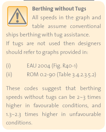
In more difficult conditions velocities may be estimated from below Figure on which five curves are given corresponding to the following navigation conditions.

a) Good berthing, sheltered;
b) Difficult berthing, sheltered;
c) Good berthing, exposed to waves and/or currents;
d) Difficult berthing, exposed to waves and/or currents;
e) Adverse berthing, exposed to waves and/or currents.

Ship size vs Berthing Speed Calculation

(2) Hydrodynamic Mass Coefficient, CM

The hydrodynamic mass coefficient allows the movement of water around the ship to be taken into account when calculating the total energy of the vessel by increasing the mass of the system. The hydrodynamic mass coefficient CM may be calculated from the following equation (BSI, 2014):

CM = 1 + 2T/B = 1.5

Where T is the draft of the vessel (m).
B is the beam of the vessel (m).

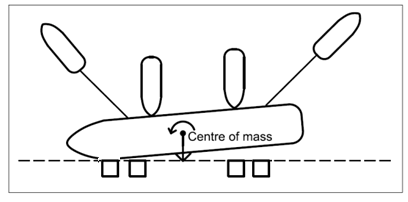
(3) Eccentricity Coefficient, CE

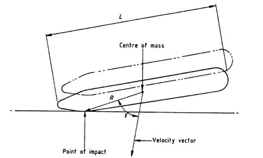
A vessel will usually berth at a certain angle and hence it turns simultaneously at the time of first impact. During this process, some of the kinetic energy of the ship is converted to turning energy and the remaining energy is transferred to the berth. The eccentricity coefficient represents the proportion of the remaining energy to the kinetic energy of the vessel at berthing. The formula for calculating the coefficient is given as follows (BSI, 2014):

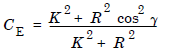
Where K is the radius of gyration of the ship.
K = (0.19Cb + 0.11) L
L is the length of the hull between perpendiculars (m).
Cb is the block coefficient
Cb = displacement (kg)/(L(m) x beam(m) x draft(m) x density of water(kg/m3))
R is the distance of the point of contact from the centre of mass (m).
γ is the angle between the line joining the point of contact to the centre of mass and the velocity vector.

4) Softness Coefficient, CS

The softness coefficient allows for the portion of the impact energy that is absorbed by the ship’s hull. Little research into energy absorption by ship hulls has taken place, but it has been generally accepted that the value of CS lies between 0.9 and 1.0. For ships, which are fitted with continuous rubber fendering, CS may be taken to be 0.9. For all other vessels CS = 1.

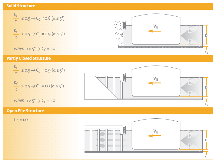
(5) Berth Configuration Coefficient / Water Cushion Effect, CC

The berth configuration coefficient allows for the portion of the ship’s energy, which is absorbed by the cushioning effect of water trapped between the ship’s hull and Wharf wall. The value Cc is between the ship’s hull and Wharf wall. The value of CC is influenced by the type of Wharf construction, and its distance from the side of the vessel, the berthing angle, the shape of the ship’s hull, and it’s under keel clearance. A value of 1.0 for CC should be used for open piled Wharf structures, and a value of Cc of between 0.8 and 1.0 is recommended for use with a solid Wharf wall.

PictureBerth Configuration Coefficient Water Cushion Effect

4.5.2 Berthing Energy Distribution

It shall be assumed that the first berthing fender will absorb 100% of total berthing energy.

Berthing Load Estimation

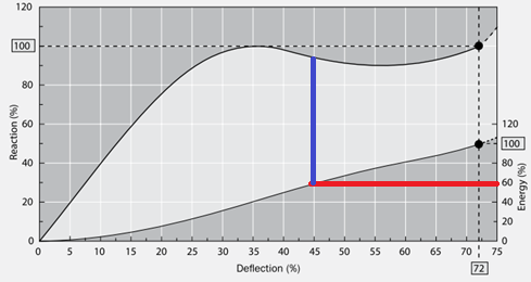
Super cone fender or other fenders shall be used to absorb berthing energy. Characteristic of fender compression and reaction force shall be used to determine compression of fenders.

According to the calculated berthing energy, the berthing load can be extracted from the generic curve of super cone fender. In below fender characteristic graph, two curves are included. Lower curve represents percentage of maximum energy absorbed by the fender vs percentage of maximum deflection of fender. Higher curve reflects percentage of maximum reaction of fender vs percentage of maximum deflection. Assuming Berthing load absorbed by one fender, we can calculate this energy in terms of fender maximum energy absorption capacity (red line). Corresponding deflection of fender can be calculated from lower graph (Blue Line). For same percentage of deflection, corresponding reaction produced can be calculated from higher curve.

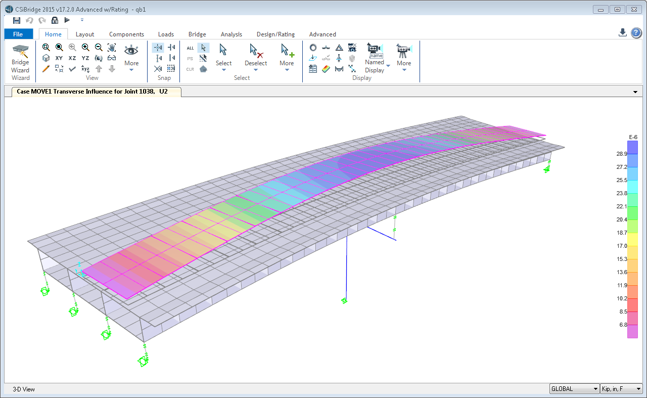
Hydrodynamic Analysis

Diffraction Radiation calculation are performed with software. This classical problem of diffraction radiation leads to the evaluation of the hydrodynamic loads
on a structure, submitted to regular waves and enable to get accurate RAOs operation of the vessel. The effect of shallow water on drift loads is considered in the analyses and provides proper drift forces on the hull (QTF, Newman Approximation). Ship hydrodynamic model shall be used which gives resultant forces bit higher than original barge and tug boat. 30 x8x3 m barge hull is modelled with windage area of 10x76x4 This arrangement represents hull with cargo windage area or tug boat with accommodation windage area.

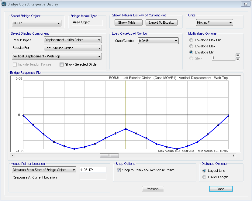
Time Domain Mooring Analysis

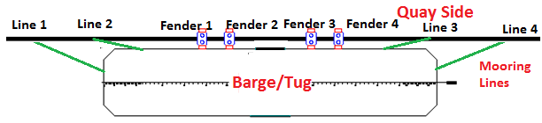
The analysis is an assessment of the loads made at the Mooring bit, fenders and the mooring lines based on a numerical model using available data. The simplified configuration of the Barge/Tug boat is modelled in Moses as per design data previously presented and based on the following assumptions

Barge/Tug boat are moored to the mooring bit using mooring ropes and resting on fenders. Barge/Tug boat is modelled with 4 mooring lines. Hull is a moving body under the action of wind wave and current. Mooring ropes are modelled as nonlinear spring. First, incidences of wind, wave and current are decided based on available metocean data. Then, time domain analyses are run for the independent wind wave and current cases for 1 hour duration to be able to decide the worst headings to study the combinations of wind wave and current.

Second, the time domain analyses for the combinations of maximum individual wind wave and current are run. The duration of the simulations are 3 hours at real time ensuring the capture of sufficient number of low frequency motions cycles.

Hydraulic Modular Trailer

A modular trailer is a series of special vehicles that is used to transport large cargos that are difficult to disassemble. The trailer is also used transport over-length goods.

The major applications of modular trailers include power stations, chemical industry, iron and steel industry and the construction industry. Modular trailers are used for mining operations because of their excellent lateral stability.

A self-propelled modular transporter without the power pack unit is similar to the hydraulic modular trailer. The main between the modular trailer and the SPMT without the PPU is that they have a different steering system.

The modular trailer uses a mechanical steering system. Another difference is that the modular trailer can be combined using a gooseneck and a drawbar.

The vehicle loading platform of a modular trailer is kept at balance when transporting goods on bumpy or rough roads in a way that the damping property is excellent.

The brace kit of the vehicle can achieve three or four brace points to ensure that the load of each point is uniform. The four points also ensure that there is no partial set.

The steering system of the modular trailer has a hydraulic planar pitman driver. The vehicle can achieve minimum turning diameter and normal drive by adjusting the hydraulic steering system and using different reasonable pitman layouts.

The supporting assemblies for the trailer part have a solid box beam structure. High performance welding steel is used to make the main frame longitudinal girder, bogie frame, steering arm, and the platform.

This form of combination is in different series include the 2-file, 3-file, and 4- file combination with drawbar. The main difference on these combinations is the type of accessories used. Each of these combinations is outlined below.

This is useful 16 panel Hydraulic Platform Transporter Reference Card is developed by me, Marco J. van Daal, and is applicable for every type of hydraulic platform transporter on the market today, both pull type as well as self propelled modular transporters (SPMT).